
In this guide, we will discuss R Normal Distribution.
In random collections of data from independent sources, it is commonly seen that the distribution of data is normal. It means that if we plot a graph with the value of the variable in the horizontal axis and counting the values in the vertical axis, then we get a bell shape curve. The curve center represents the mean of the data set. In the graph, fifty percent of the value is located to the left of the mean. And the other fifty percent to the right of the graph. This is referred to as the normal distribution.
R allows us to generate normal distribution by providing the following functions:

These function can have the following parameters:
| S.No | Parameter | Description |
|---|---|---|
| 1. | x | It is a vector of numbers. |
| 2. | p | It is a vector of probabilities. |
| 3. | n | It is a vector of observations. |
| 4. | mean | It is the mean value of the sample data whose default value is zero. |
| 5. | sd | It is the standard deviation whose default value is 1. |
Let’s start understanding how these functions are used with the help of examples.
dnorm():Density
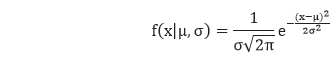
The norm() function of R calculates the height of the probability distribution at each point for a given mean and standard deviation. The probability density of the normal distribution is:
Example
# Creating a sequence of numbers between -1 and 20 incrementing by 0.2.
x <- seq(-1, 20, by = .2)
# Choosing the mean as 2.0 and standard deviation as 0.5.
y <- dnorm(x, mean = 2.0, sd = 0.5)
# Giving a name to the chart file.
png(file = "dnorm.png")
#Plotting the graph
plot(x,y)
# Saving the file.
dev.off()
Output:

pnorm():Direct Look-Up
The norm() function is also known as the “Cumulative Distribution Function”. This function calculates the probability of normally distributed random numbers, which is less than the value of a given number. The cumulative distribution is as follows:
f(x)=P(X≤x)
Example
# Creating a sequence of numbers between -1 and 20 incrementing by 0.2.
x <- seq(-1, 20, by = .1)
# Choosing the mean as 2.0 and standard deviation as 0.5.
y <- pnorm(x, mean = 2.0, sd = 0.5)
# Giving a name to the chart file.
png(file = "pnorm.png")
#Plotting the graph
plot(x,y)
# Saving the file.
dev.off()
Output:

qnorm():Inverse Look-Up
The qnorm() function takes the probability value as an input and calculates a number whose cumulative value matches with the probability value. The cumulative distribution function and the inverse cumulative distribution function are related by
Example
# Creating a sequence of numbers between -1 and 20 incrementing by 0.2.
x <- seq(0, 1, by = .01)
# Choosing the mean as 2.0 and standard deviation as 0.5.
y <- qnorm(x, mean = 2.0, sd = 0.5)
# Giving a name to the chart file.
png(file = "qnorm.png")
#Plotting the graph
plot(y,x)
# Saving the file.
dev.off()
Output:

rnorm():Random variates
The rnorm() function is used for generating normally distributed random numbers. This function generates random numbers by taking the sample size as an input. Let’s see an example in which we draw a histogram for showing the distribution of the generated numbers.
Example
# Creating a sequence of numbers between -1 and 20 incrementing by 0.2.
x <- rnorm(1500, mean=80,  sd=15 )
# Giving a name to the chart file.
png(file = "rnorm.png")
#Creating histogram
hist(x,probability =TRUE,col="red",border="black")
# Saving the file.
dev.off()
Output:

Next Topic; Click Here